Free Energy Reinforcement Learning Implementation

Question

I've been trying to implement the algorithm described here, and then test it on the "large action task" described in the same paper.

Overview of the algorithm:

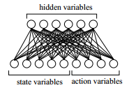
In brief, the algorithm uses an RBM of the form shown below to solve reinforcement learning problems by changing its weights such that the free energy of a network configuration equates to the reward signal given for that state-action pair.

To select an action, the algorithm performs Gibbs sampling while holding the state variables fixed. With enough time, this produces the action with the lowest free energy, and thus the highest reward for the given state.

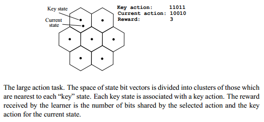
Overview of the large action task:

Overview of the author's guidelines for implementation:

A restricted Boltzmann machine with 13 hidden variables was trained on an instantiation of the large action task with a 12-bit state space and a 40-bit action space. Thirteen key states were randomly selected. The network was run for 12 000 actions with a learning rate going from 0.1 to 0.01 and temperature going from 1.0 to 0.1 exponentially over the course of training. Each iteration was initialized with a random state. Each action selection consisted of 100 iterations of Gibbs sampling.

Important omitted details:

• Were bias units needed?

• Was weight decay needed? And if so, L1 or L2?

• Was a sparsity constraint needed for the weights and/or activations?

• Was there a modification of the gradient descent? (e.g. momentum)

• What meta-parameters were needed for these additional mechanisms?

My implementation:

I initially assumed the authors' used no mechanisms other than those described in the guidelines, so I tried training the network without bias units. This led to near chance performance and was my first clue to the fact that some mechanisms used must have been deemed 'obvious' by the authors and thus omitted.

I played around with the various omitted mechanisms mentioned above, and got my best results by using:

• softmax hidden units

• momentum of .9 (.5 until 5th iteration)

• bias units for the hidden and visible layers

• a learning rate 1/100th of that listed by the authors.

• l2 weight decay of .0002

But even with all of these modifications, my performance on the task was generally around an average reward of 28 after 12000 iterations.

Code for each iteration:

%%%%%%%%% START POSITIVE PHASE %%%%%%%%%%%%%%%%%%%%%%%%%%%%%%%%%%%%%%%%%%%%%%%%%%% 

data = [batchdata(:,:,(batch)) rand(1,numactiondims)>.5]; 

poshidprobs = softmax(data*vishid + hidbiases); 

%%%%%%%%% END OF POSITIVE PHASE %%%%%%%%%%%%%%%%%%%%%%%%%%%%%%%%%%%%%%%%%%%%%%%%% 

hidstates = softmax_sample(poshidprobs); 

%%%%%%%%% START ACTION SELECTION PHASE %%%%%%%%%%%%%%%%%%%%%%%%%%%%%%%%%%%%%%%%%%%%%%%%%% 

if test [negaction poshidprobs] = choose_factored_action(data(1:numdims),hidstates,vishid,hidbiases,visbiases,cdsteps,0); 

else [negaction poshidprobs] = choose_factored_action(data(1:numdims),hidstates,vishid,hidbiases,visbiases,cdsteps,temp); 

end data(numdims+1:end) = negaction > rand(numcases,numactiondims); 

if mod(batch,100) == 1 disp(poshidprobs); 

disp(min(~xor(repmat(correct_action(:,(batch)),1,size(key_actions,2)), key_actions(:,:)))); 

end posprods = data' * poshidprobs; 

poshidact = poshidprobs;

posvisact = data; 

%%%%%%%%% END OF ACTION SELECTION PHASE %%%%%%%%%%%%%%%%%%%%%%%%%%%%%%%%%%%%%%%%%%%%%%%%%% 

if batch>5, momentum=.9; 

else momentum=.5; 

end; 

%%%%%%%%% UPDATE WEIGHTS AND BIASES %%%%%%%%%%%%%%%%%%%%%%%%%%%%%%%%%%%%%%%%%%%%%%% 

F=calcF_softmax2(data,vishid,hidbiases,visbiases,temp);

Q = -F; 

action = data(numdims+1:end); 

reward = maxreward - sum(abs(correct_action(:,(batch))' - action)); 

if correct_action(:,(batch)) == correct_action(:,1) 

reward_dataA = [reward_dataA reward]; 

Q_A = [Q_A Q]; 

else 

reward_dataB = [reward_dataB reward]; 

Q_B = [Q_B Q]; 

end reward_error = sum(reward - Q); 

rewardsum = rewardsum + reward; 

errsum = errsum + abs(reward_error); 

error_data(ind) = reward_error; 

reward_data(ind) = reward; 

Q_data(ind) = Q; 

vishidinc = momentum*vishidinc + ... epsilonw*( (posprods*reward_error)/numcases - weightcost*vishid); 

visbiasinc = momentum*visbiasinc + (epsilonvb/numcases)*((posvisact)*reward_error - weightcost*visbiases);

hidbiasinc = momentum*hidbiasinc + (epsilonhb/numcases)*((poshidact)*reward_error - weightcost*hidbiases); 

vishid = vishid + vishidinc; 

hidbiases = hidbiases + hidbiasinc; 

visbiases = visbiases + visbiasinc; 

%%%%%%%%%%%%%%%% END OF UPDATES %%%%%%%%%%%%%%%%%%%%%%%%%%%%%%%%%%%%%%%%%%%%%%%%%%%%

What I'm asking for:

So, if any of you can get this algorithm to work properly (the authors claim to average ~40 rewards after 12000 iterations), I'd be extremely grateful.

If my code appears to be doing something obviously wrong, then calling attention to that would also constitute a great answer.

I'm hoping that what the authors left out is indeed obvious to someone with more experience with energy-based learning than myself, in which case, simply point out what needs to be included in a working implementation.

Answer 1

Good actions will become more probable under this model, and bad actions will become less probable under the model. Although finding optimal actions would still be difficult for large problems, selecting an action with a probability that approximately equals to the probability under the Boltzmann distribution can normally be done with a small number of iterations of MCMC(Markov chain Monte Carlo) sampling. MCMC sampling is the type of sampling which contains the methods which contain a class of algorithms for sampling from a probability distribution.

In this, if we let the MCMC sampling to meet to the equilibrium distribution then we can able to draw unbiased samples from the Boltzmann exploration policy at a particular temperature. 

The network was run for 12 000 actions with a learning rate going from 0.1 to 0.01 and temperature going from 1.0 to 0.1 exponentially over the course of training. Each iteration was initialized with a random state. Each action that is selected consisted of 100 iterations of Gibbs sampling. For each execution of the method, the task was repeated 10 times. The competing methods also had learning rates and (in the case of the backprop network) exploration schedules. The backprop network used a learning rate going from 0.005 to 0.004, and a ε-greedy exploration strategy going from 1 to 0 linearly over the course of the task. The direct policy method used a learning rate going from 0.1 to 0.01 over the course of the task. All the learning parameters that were selected by trial and error during preliminary experiments, with the best-performing parameters reported in the method.

If you wish to learn about Implementations of Reinforcement Learning then visit this Reinforcement Learning Certification Training.