Question

How can I use Tableau to create a heatmap?

I have the data below where Below is how the data looks like. Each D* refers to one of the three variables that are all correlated against each other. There are 3 instances of each D* variable. When the same variables are against each other in that case 'NA'.

    D1  D1  D1  D2  D2  D2  D3  D3  D3
D1         
D1 
D1 
D2  0.3 0.3 0.3
D2  0.4 0.2 -0.2   
D2  0.1 0.3 0.4    
D3  0.6 0.6 0.6 0.2 0.2 0.2
D3  0.6 0.8 0.9 0.4 0.2 -0.2   
D3  0.7 0.7 0.7 0   0.2 0.2
I want to make a heatmap from this data where the correalation values (coefficients) are converted to colors. Step-by-step, what can I do to reformat or otherwise the data to achieve this?

Answer 1

Step 1: You can create an Excel Spreadsheet with the table exactly as you provided above, but rename the different D* instances by adding a, b and c as required. Save the excel spreadsheet.

Step 2: Open Tableau and connect to the Excel file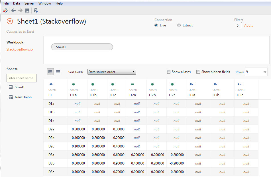

Step 3: Select columns D1a to D3c

Step 4: You need to hover your mouse and click on the drop down arrow and select pivot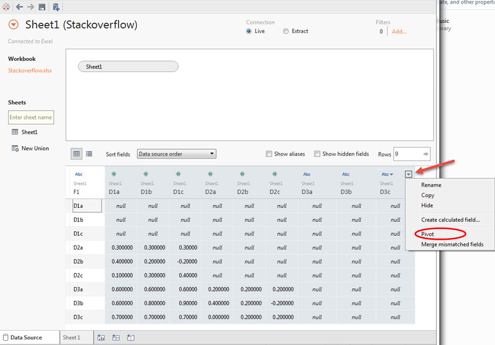

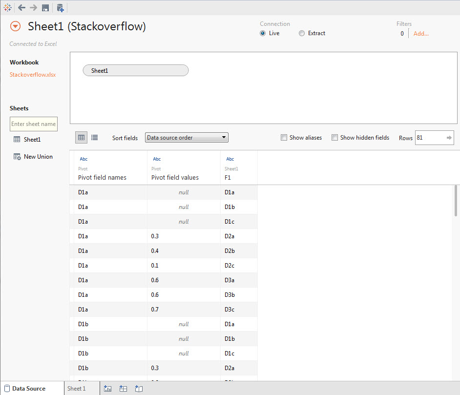
Step 5: Now, Double click on F1, Pivot field names and Pivot field values and rename as appropriate. Note the slight variations in the names.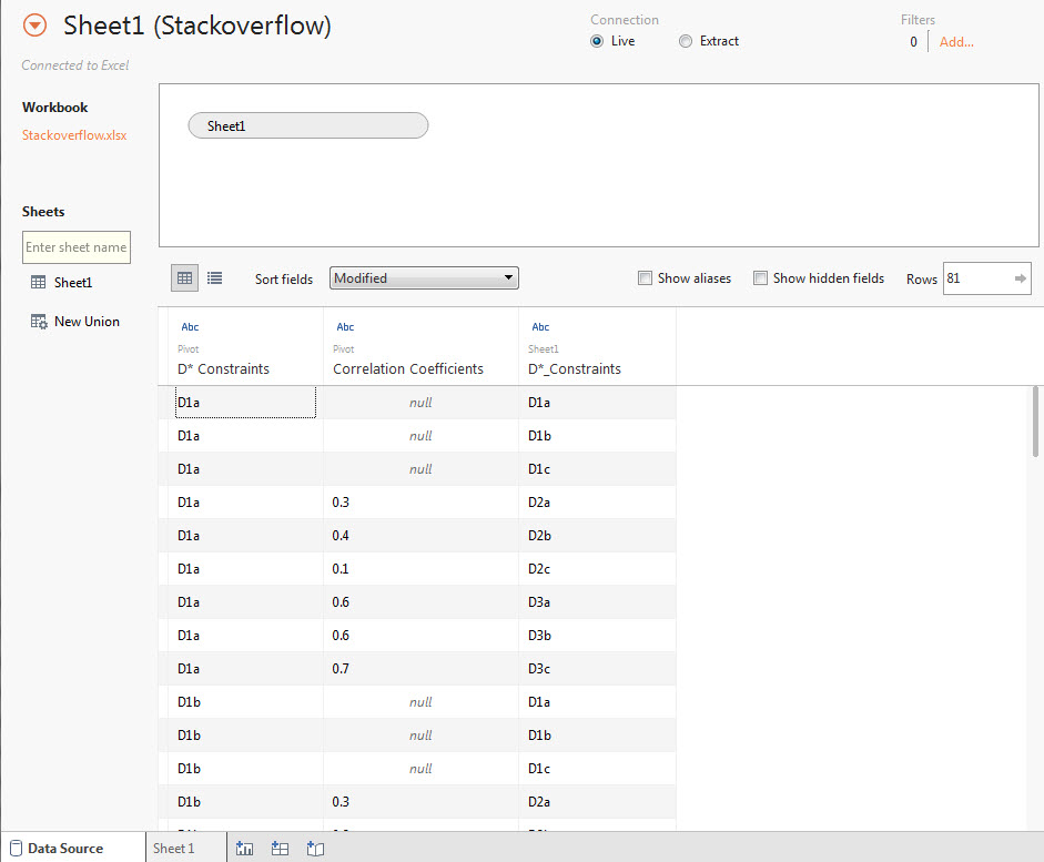

Step 6: Change the data type for correlation coefficients. Click on Abc and change as shown. Click on Sheet 1 when you are done.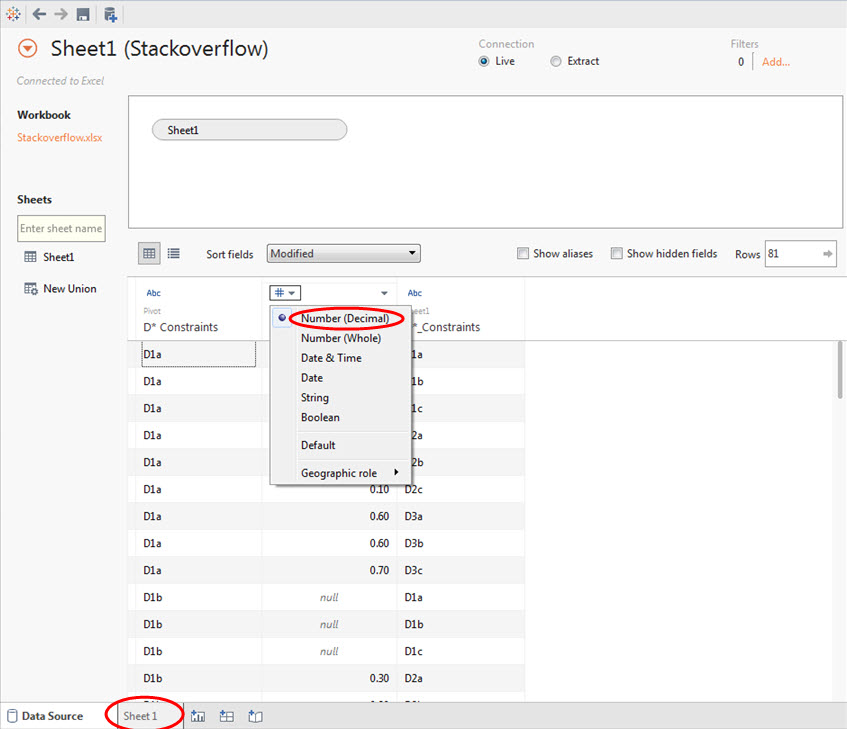

Step 7: Now, Right click on Correlation Coefficients and click Convert to measure.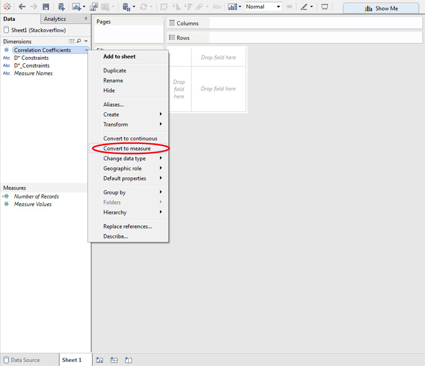

Step 8: As shown in the image, drag the different D* fields to the row and column shelves Drag Correlation Coefficients onto the Color Marks card.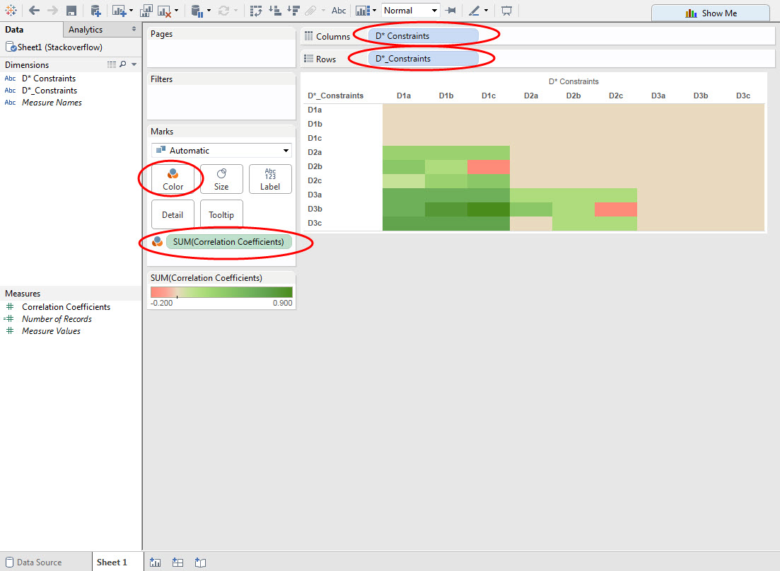

Step 9: As shown in the image, Click on “Abc” at the top. Hover your mouse and click on the drop down arrow and Edit colors.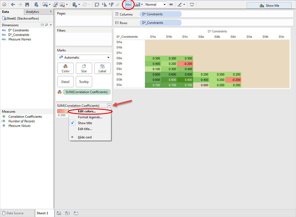

Step 10: Choose the options shown below. Feel free to use this format if you wish.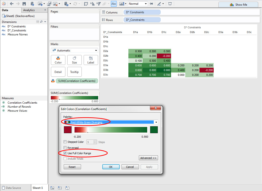

Step 11: Click on the end member green color and select the lighter green color as shown. Deselect “Use Full Color Range”. Click OK.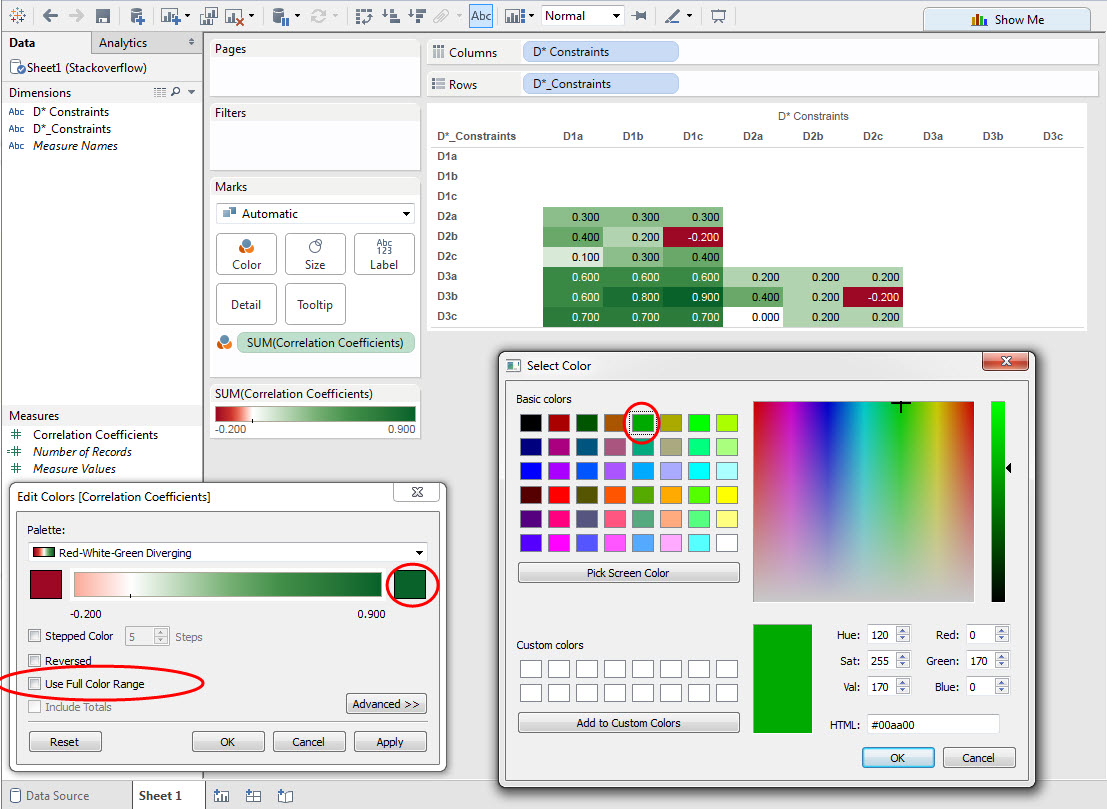

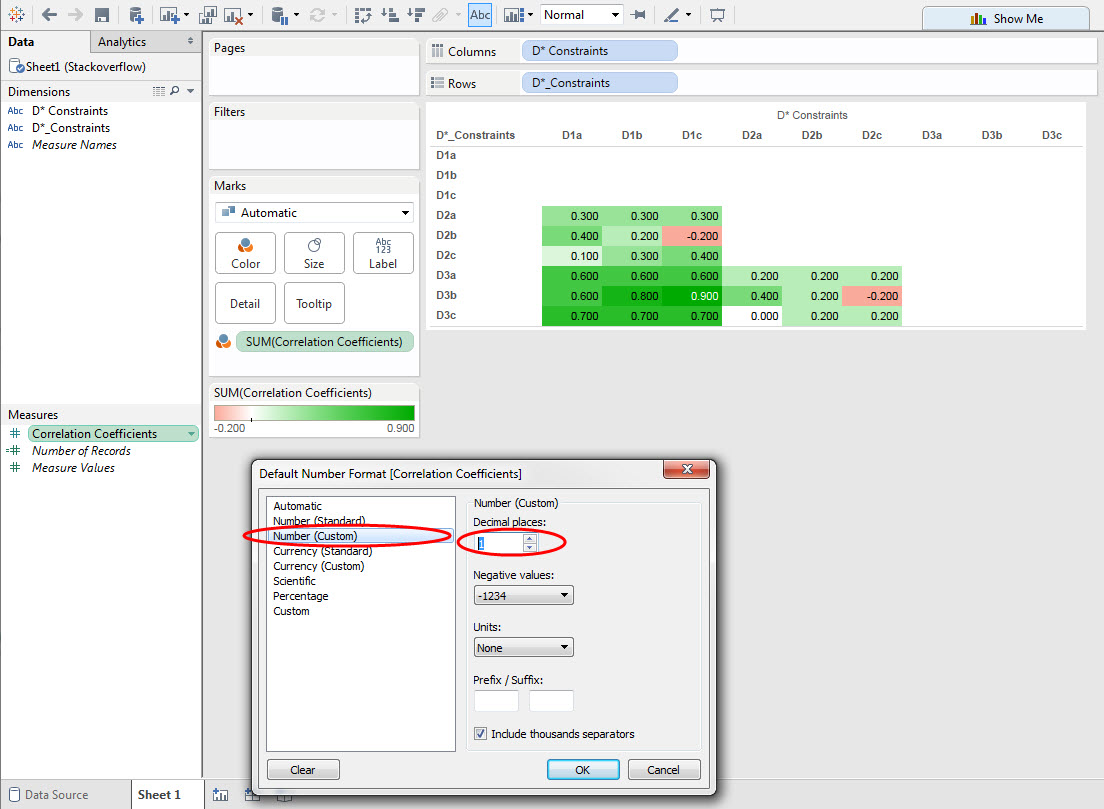
Step 12: Format the Correlation Coefficients as shown.

Step 13: You are done with building your Tableau visualization.\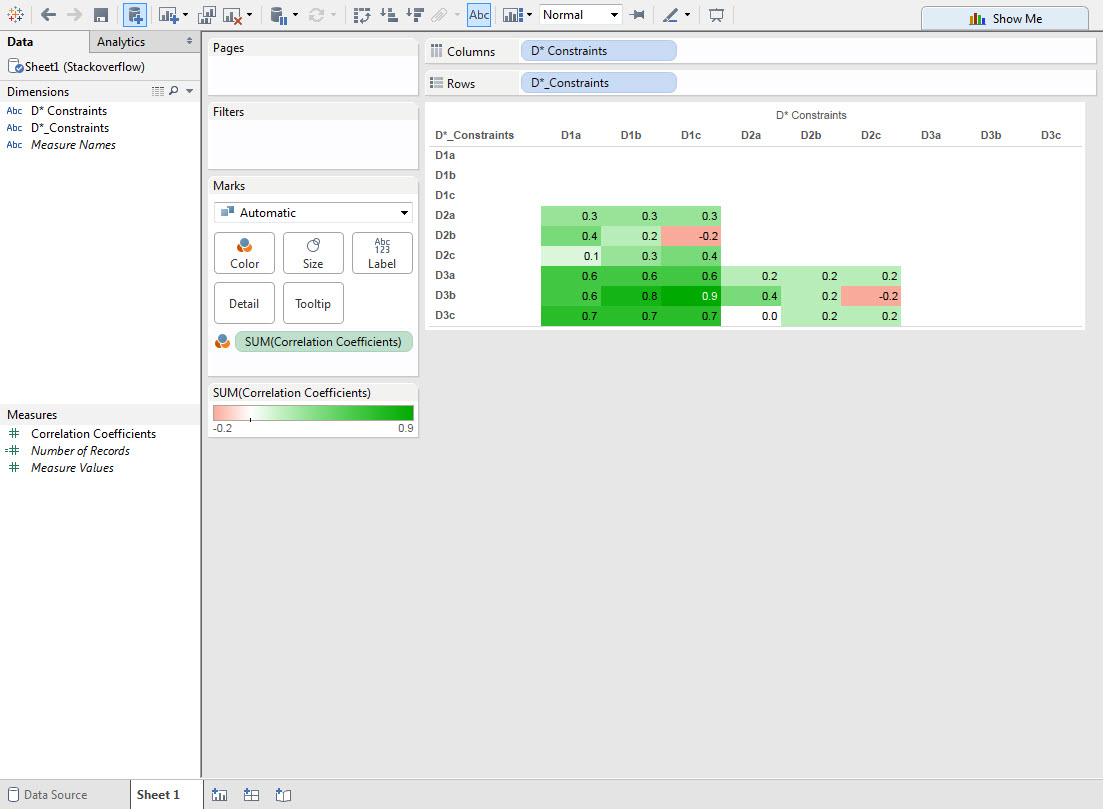

Interested to learn about Tableau from top experts? Enroll in Tableau Course to get expert guidance.